Grouped Data Analysis

Our customly-defined function provides a newly grouped dataset that compresses the 12 million data points into ~80 subtotals that are easier to represent graphically. The total_walltime field represents the total amount of walltime consumed during that month in hours. Likewise, the two other walltime fields represent the total stratified by jobs with either successful or failed exit status. The number of unique users is based on unique username. The dataset can be explored below using the interactive table.

Monthly Datatables

Helix

helix.monthly = generate_monthly(helix.full)

datatable(helix.monthly, options = list(pageLength = 5))

print(dfSummary(helix.monthly, 
                #plain.ascii = FALSE, style="grid", 
                graph.magnif = 0.75, valid.col=FALSE), 
      method='render')

Data Frame Summary

Dimensions: 78 x 9
Duplicates: 0

Variable

Stats / Values

Freqs (% of Valid)

Graph

Missing

month [character]

1. 2014-09 2. 2014-10 3. 2014-11 4. 2014-12 5. 2015-01 6. 2015-02 7. 2015-03 8. 2015-04 9. 2015-05 10. 2015-06 [ 68 others ]

1	(	1.3%	)
1	(	1.3%	)
1	(	1.3%	)
1	(	1.3%	)
1	(	1.3%	)
1	(	1.3%	)
1	(	1.3%	)
1	(	1.3%	)
1	(	1.3%	)
1	(	1.3%	)
68	(	87.2%	)

0 (0.0%)

total_walltime [numeric]

Mean (sd) : 60959054 (216866247) min < med < max: 402.4 < 10859427 < 1807638505 IQR (CV) : 14769055 (3.6)

78 distinct values

0 (0.0%)

num.successful.jobs [integer]

Mean (sd) : 137694.2 (152316.4) min < med < max: 221 < 99585 < 992595 IQR (CV) : 144684.8 (1.1)

78 distinct values

0 (0.0%)

num.failed.jobs [integer]

Mean (sd) : 16644.3 (16903.8) min < med < max: 15 < 13505 < 127885 IQR (CV) : 14795.2 (1)

78 distinct values

0 (0.0%)

failed.walltime [numeric]

Mean (sd) : 11532271 (37711684) min < med < max: 111.8 < 2918231 < 255457234 IQR (CV) : 3106090 (3.3)

78 distinct values

0 (0.0%)

successful.walltime [numeric]

Mean (sd) : 49426782 (206508199) min < med < max: 290.6 < 7573931 < 1790575341 IQR (CV) : 13343934 (4.2)

78 distinct values

0 (0.0%)

unique.users [integer]

Mean (sd) : 77.3 (33.1) min < med < max: 3 < 72.5 < 149 IQR (CV) : 44.8 (0.4)

62 distinct values

0 (0.0%)

used.memory [numeric]

Mean (sd) : 675610277888 (841328540890) min < med < max: 780799804 < 408300914260 < 4.339691e+12 IQR (CV) : 581456370702 (1.2)

78 distinct values

0 (0.0%)

total.jobs [integer]

Mean (sd) : 154338.4 (159688.8) min < med < max: 236 < 118553 < 1023465 IQR (CV) : 162040 (1)

78 distinct values

0 (0.0%)

Generated by summarytools 0.9.8 (R version 4.0.4)
2021-03-15

Cadillac

cadillac.monthly = generate_monthly(cadillac.full)

datatable(cadillac.monthly, options = list(pageLength = 5))

print(dfSummary(cadillac.monthly, 
          #plain.ascii = FALSE, style="grid", 
          graph.magnif = 0.75, valid.col=FALSE),
      method='render')

Data Frame Summary

Dimensions: 82 x 9
Duplicates: 0

Variable

Stats / Values

Freqs (% of Valid)

Graph

Missing

month [character]

1. 2014-04 2. 2014-05 3. 2014-06 4. 2014-07 5. 2014-08 6. 2014-09 7. 2014-10 8. 2014-11 9. 2014-12 10. 2015-01 [ 72 others ]

1	(	1.2%	)
1	(	1.2%	)
1	(	1.2%	)
1	(	1.2%	)
1	(	1.2%	)
1	(	1.2%	)
1	(	1.2%	)
1	(	1.2%	)
1	(	1.2%	)
1	(	1.2%	)
72	(	87.8%	)

0 (0.0%)

total_walltime [numeric]

Mean (sd) : 4232766 (9829658) min < med < max: 322 < 2207462 < 86587820 IQR (CV) : 3163944 (2.3)

82 distinct values

0 (0.0%)

num.successful.jobs [integer]

Mean (sd) : 37168 (38973.1) min < med < max: 115 < 27641.5 < 167333 IQR (CV) : 33838.5 (1)

82 distinct values

0 (0.0%)

num.failed.jobs [integer]

Mean (sd) : 5185.3 (4191) min < med < max: 183 < 4296 < 25793 IQR (CV) : 3525.2 (0.8)

82 distinct values

0 (0.0%)

failed.walltime [numeric]

Mean (sd) : 887928.2 (1825153) min < med < max: 4.7 < 350939.4 < 13246188 IQR (CV) : 681140.8 (2.1)

82 distinct values

0 (0.0%)

successful.walltime [numeric]

Mean (sd) : 3344838 (8365428) min < med < max: 174 < 1754213 < 73341632 IQR (CV) : 2020438 (2.5)

82 distinct values

0 (0.0%)

unique.users [integer]

Mean (sd) : 33.7 (15.9) min < med < max: 2 < 39 < 62 IQR (CV) : 20.2 (0.5)

39 distinct values

0 (0.0%)

used.memory [numeric]

Mean (sd) : 207387316253 (171705189017) min < med < max: 455756024 < 165342092946 < 781106399544 IQR (CV) : 215429808788 (0.8)

82 distinct values

0 (0.0%)

total.jobs [integer]

Mean (sd) : 42353.3 (40774.6) min < med < max: 4431 < 32707 < 178261 IQR (CV) : 40131.2 (1)

82 distinct values

0 (0.0%)

Generated by summarytools 0.9.8 (R version 4.0.4)
2021-03-15

The monthly datasets can be found in data/[cluster].monthly.rds in GitHub.

Job Counts

Right away, we may use this to produce some graphical representations of the usage for both Helix and Cadillac.

Below is a plot of all the total job count. The slider below can be used to adjust the time scale. The red shaded area on the graph represents Sumner came online.

Predictions using Error/Trend/Seasonality (ETS) Modeling

Job Count Predictions

In order to quantify the rate of depreciation in job count, we will apply an exponential smoothing model to our time series data in order to extract any seasonality, trend, or error. For our smoothing, we will use the Holt-Winters method because it is a simplistic exponential smoothing method that is very agnostic to underlying trends (which we know exist due to our observations of the graphs above).

Below is a model of the total job counts per month. We will leave the question of whether or not the error, trend, and seasonality is multiplicative or additive up to the algorithm to determine. In order to verify this is a good model, we will also check the residuals.

ETS Models

Helix

helix.hw = ets(helix.jobs.ts, model = "ZZZ")
#Nerd Stuff
summary(helix.hw)
#> ETS(M,Ad,M) 
#> 
#> Call:
#>  ets(y = helix.jobs.ts, model = "ZZZ") 
#> 
#>   Smoothing parameters:
#>     alpha = 0.2423 
#>     beta  = 0.0216 
#>     gamma = 0.0077 
#>     phi   = 0.98 
#> 
#>   Initial states:
#>     l = -6016.0442 
#>     b = 6698.8325 
#>     s = 0.594 1.487 1.8706 0.8337 1.8708 0.6677
#>            0.4796 1.4908 0.6294 0.5856 0.8866 0.6043
#> 
#>   sigma:  0.6369
#> 
#>      AIC     AICc      BIC 
#> 2085.374 2096.968 2127.795 
#> 
#> Training set error measures:
#>                     ME     RMSE      MAE      MPE     MAPE      MASE       ACF1
#> Training set -22621.08 153837.8 88048.56 -46.6737 72.50789 0.6993508 0.04626555

checkresiduals(helix.hw, plot=TRUE)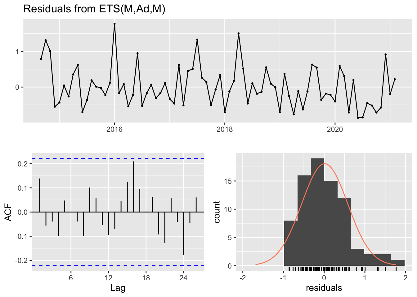

#> 
#>  Ljung-Box test
#> 
#> data:  Residuals from ETS(M,Ad,M)
#> Q* = 15.202, df = 3, p-value = 0.001652
#> 
#> Model df: 17.   Total lags used: 20

Cadillac

cadillac.hw = ets(cadillac.jobs.ts, model = "ZZZ")
#Nerd Stuff
summary(cadillac.hw)
#> ETS(M,Ad,N) 
#> 
#> Call:
#>  ets(y = cadillac.jobs.ts, model = "ZZZ") 
#> 
#>   Smoothing parameters:
#>     alpha = 0.8342 
#>     beta  = 0.0122 
#>     phi   = 0.9738 
#> 
#>   Initial states:
#>     l = -37544.0003 
#>     b = 13709.6416 
#> 
#>   sigma:  0.6111
#> 
#>      AIC     AICc      BIC 
#> 1996.003 1997.123 2010.444 
#> 
#> Training set error measures:
#>                     ME    RMSE      MAE      MPE     MAPE      MASE        ACF1
#> Training set -4406.729 36085.6 23186.32 -54.5343 89.54353 0.5850586 -0.06897187

checkresiduals(cadillac.hw, plot=TRUE)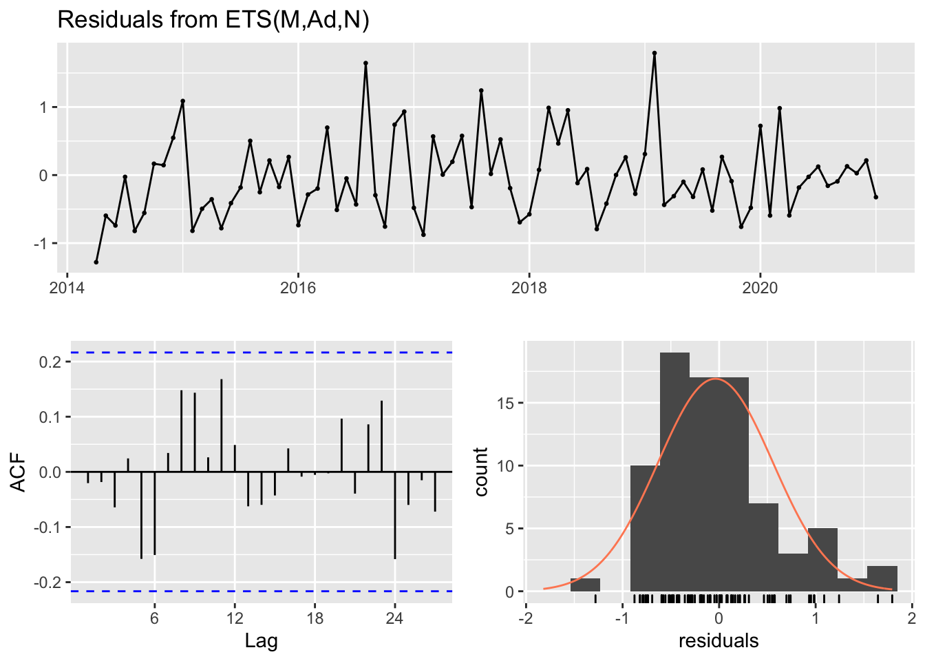

#> 
#>  Ljung-Box test
#> 
#> data:  Residuals from ETS(M,Ad,N)
#> Q* = 13.027, df = 11, p-value = 0.2916
#> 
#> Model df: 5.   Total lags used: 16

We will now use this to create a forecast of our future observations on both Helix and Cadillac. Using our model, we can construct a realistic upper limit (within 95% confidence) for the number of jobs on each cluster for the next 12 months. The area shaded in blue represents the prediction.

helix.jobs.ts.predict = ts(c(helix.monthly$total.jobs, forecast(helix.hw,h=12)$upper[,2]), start = c(2014,9), frequency = 12)
cadillac.jobs.ts.predict = ts(c(cadillac.monthly$total.jobs, forecast(cadillac.hw,h=12)$upper[,2]), start = c(2014,4), frequency=12)
jobs.ts.predict = cbind(helix.jobs.ts.predict,cadillac.jobs.ts.predict)
dygraph(jobs.ts.predict, main="Total Jobs per Month") %>% 
  dySeries("helix.jobs.ts.predict", label="Helix") %>%
  dySeries("cadillac.jobs.ts.predict", label="Cadillac") %>%
  dyAnnotation("2019-07-01", text="EOL", attachAtBottom = TRUE, width=40) %>%
  dyAxis("y", label="Total jobs ended") %>%
  dyOptions(axisLineWidth = 1.5, fillGraph = TRUE) %>%
  dyShading(from="2019-12-20", to="2021-02-01", color = "#FFE6E6") %>%
  dyShading(from="2021-02-02", to="2022-02-01", color = "#aad8e6") %>%
  dyRangeSelector()

As we can see from this graph, Cadillac looks like it will confidently never rise to levels even seen when it was declared EOL in July 2019. Just by data alone, however, we cannot say for certain if Helix will “die” based on this model. In fact, if we look at the p-value for the Ljung-Box test on the Helix model, we see that there is a 99.9% confidence that there is information that is missing from the model. For this new model, let’s look at one that is more “local” – one that is trained on data since it was declared EOL.

helix.eol.hw = ets(window(helix.jobs.ts, start = c(2019,7)), model = "ZZZ")
checkresiduals(helix.eol.hw)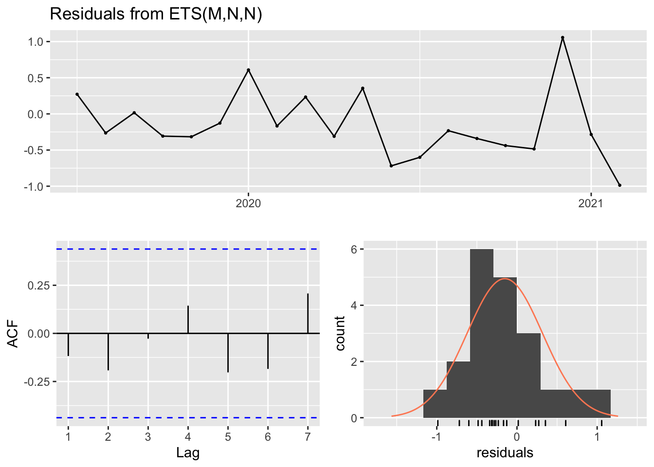

#> 
#>  Ljung-Box test
#> 
#> data:  Residuals from ETS(M,N,N)
#> Q* = 3.0216, df = 3, p-value = 0.3883
#> 
#> Model df: 2.   Total lags used: 5


helix.eol = ts(c(window(helix.jobs.ts, start = c(2019,7)), forecast(helix.eol.hw,h=12)$upper[,2]), start = c(2019,7), frequency = 12)

Residuals show that the model fits relatively well, however falls a little short towards the end of the data where the job count starts to fall off drastically.

dygraph(helix.eol, main = "Helix Predictions Trained on EOL Window Data") %>%
  dyAxis("y", label="Total jobs ended") %>%
  dyOptions(axisLineWidth = 1.5, fillGraph = TRUE) %>%
  dyShading(from="2021-02-02", to="2022-02-01", color = "#aad8e6") %>%
  dyRangeSelector()

Unique User Count Predictions

This metric measures the number of unique users that logged into the clusters per month. This number fluctuates greatly from day to day (when grouped by day \(\mu = 23.53\), \(\sigma = 13.64\) users) so visualizations in terms of day will be relatively useless. Once again, the red shaded area represents when Sumner came online.

helix.users.ts = ts(helix.monthly$unique.users, start = c(2014,9), frequency = 12)
cadillac.users.ts = ts(cadillac.monthly$unique.users, start = c(2014,4), frequency=12)
users.ts = cbind(helix.users.ts,cadillac.users.ts)
dygraph(users.ts, main="Unique Users per Month") %>% 
  dySeries("helix.users.ts", label="Helix") %>%
  dySeries("cadillac.users.ts", label="Cadillac") %>%
  dyOptions(stackedGraph=TRUE) %>%
  dyAnnotation("2019-07-01", text="EOL", attachAtBottom = TRUE, width=40) %>%
  dyAxis("y", label="Users") %>%
  dyOptions(axisLineWidth = 1.5, fillGraph = TRUE) %>%
  dyShading(from="2019-12-20", to="2021-02-01", color = "#FFE6E6") %>%
  dyRangeSelector()

Similarly to before, we will perform an exponential smoothing model (Holt-Winters) on the unique user data.

Users Model

Helix

helix.users.hw = ets(helix.users.ts, model = "ZZZ")
summary(helix.users.hw)
#> ETS(A,N,N) 
#> 
#> Call:
#>  ets(y = helix.users.ts, model = "ZZZ") 
#> 
#>   Smoothing parameters:
#>     alpha = 0.9999 
#> 
#>   Initial states:
#>     l = 2.9527 
#> 
#>   sigma:  10.2989
#> 
#>      AIC     AICc      BIC 
#> 707.5951 707.9194 714.6652 
#> 
#> Training set error measures:
#>                      ME     RMSE      MAE       MPE     MAPE      MASE       ACF1
#> Training set 0.01346803 10.16601 7.654612 -8.861156 20.14833 0.2694424 0.07555727

checkresiduals(helix.users.hw)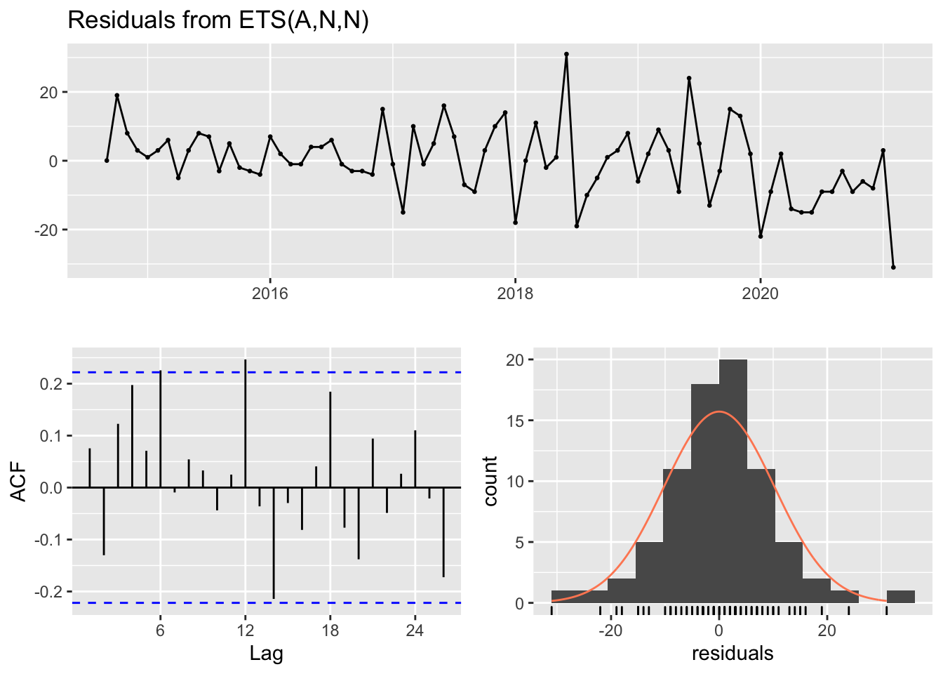

#> 
#>  Ljung-Box test
#> 
#> data:  Residuals from ETS(A,N,N)
#> Q* = 22.946, df = 14, p-value = 0.06115
#> 
#> Model df: 2.   Total lags used: 16

Cadillac

cadillac.users.hw = ets(cadillac.users.ts, model = "ZZZ")
summary(cadillac.users.hw)
#> ETS(A,N,N) 
#> 
#> Call:
#>  ets(y = cadillac.users.ts, model = "ZZZ") 
#> 
#>   Smoothing parameters:
#>     alpha = 0.7103 
#> 
#>   Initial states:
#>     l = 14.6363 
#> 
#>   sigma:  6.7237
#> 
#>      AIC     AICc      BIC 
#> 677.8507 678.1584 685.0708 
#> 
#> Training set error measures:
#>                      ME     RMSE      MAE       MPE     MAPE      MASE        ACF1
#> Training set -0.2041583 6.641188 4.972567 -8.389144 21.60065 0.3783475 0.008221298

checkresiduals(cadillac.users.hw)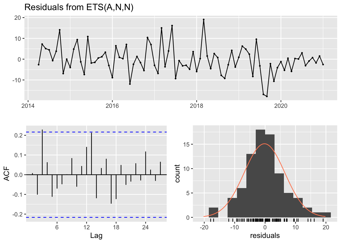

#> 
#>  Ljung-Box test
#> 
#> data:  Residuals from ETS(A,N,N)
#> Q* = 17.548, df = 14, p-value = 0.2282
#> 
#> Model df: 2.   Total lags used: 16

And now we will once again create a 95% confidence upper bound prediction for the number of unique users per month for each cluster.

helix.users.ts.predict = ts(c(helix.monthly$unique.users, forecast(helix.users.hw,h=12)$upper[,2]), start = c(2014,9), frequency = 12)
cadillac.users.ts.predict = ts(c(cadillac.monthly$unique.users, forecast(cadillac.users.hw,h=12)$upper[,2]), start = c(2014,4), frequency=12)
users.ts.predict = cbind(helix.users.ts.predict,cadillac.users.ts.predict)
dygraph(users.ts.predict, main="Unique Users per Month (12 mo. Prediction)") %>% 
  dySeries("helix.users.ts.predict", label="Helix") %>%
  dySeries("cadillac.users.ts.predict", label="Cadillac") %>%
  dyAnnotation("2019-07-01", text="EOL", attachAtBottom = TRUE, width=40) %>%
  dyAxis("y", label="Users") %>%
  dyOptions(axisLineWidth = 1.5, fillGraph = TRUE) %>%
  dyShading(from="2019-12-20", to="2021-02-01", color = "#FFE6E6") %>%
  dyShading(from="2021-02-02", to="2022-02-01", color = "#aad8e6") %>%
  dyRangeSelector()

Just like before, we see that the predictions may vary wildly due to training on the whole dataset. We will subset our training set, and make a new prediction.

Localized Models

Helix

helix.users.eol.hw = ets(window(helix.users.ts, start = c(2019,7)), model = "ZZZ")
helix.users.eol = ts(c(window(helix.users.ts, start = c(2019,7)), forecast(helix.users.eol.hw,h=12)$upper[,2]), start = c(2019,7), frequency = 12)
checkresiduals(helix.users.eol.hw)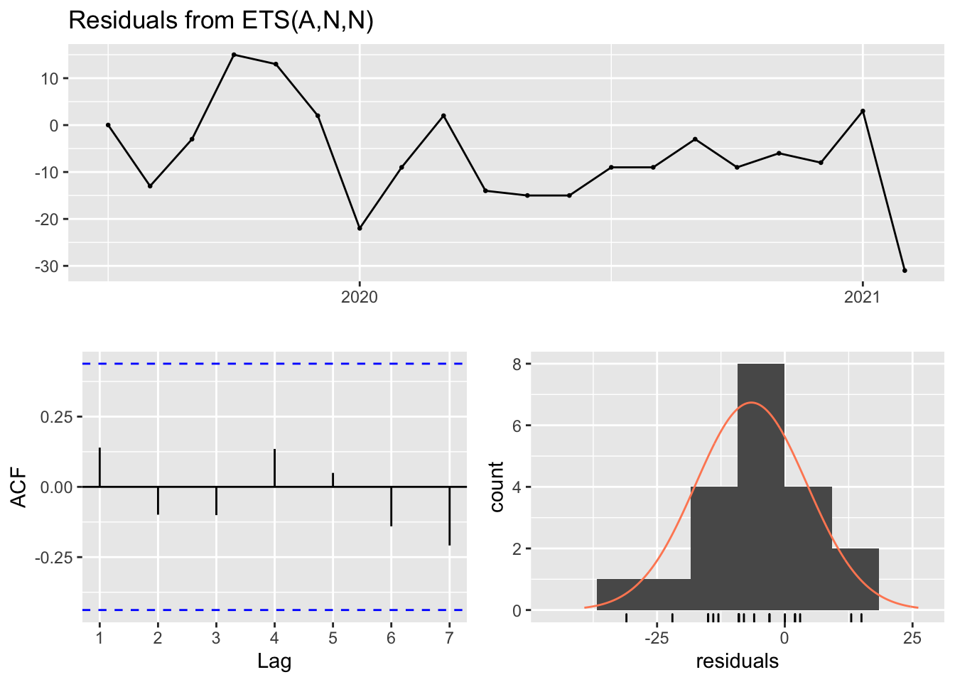

#> 
#>  Ljung-Box test
#> 
#> data:  Residuals from ETS(A,N,N)
#> Q* = 1.5265, df = 3, p-value = 0.6762
#> 
#> Model df: 2.   Total lags used: 5

Cadillac

cadillac.users.eol.hw = ets(window(cadillac.users.ts, start = c(2019,7)), model = "ZZZ")
cadillac.users.eol = ts(c(window(cadillac.users.ts, start = c(2019,7)), forecast(cadillac.users.eol.hw,h=12)$upper[,2]), start = c(2019,7), frequency = 12)
checkresiduals(cadillac.users.eol.hw)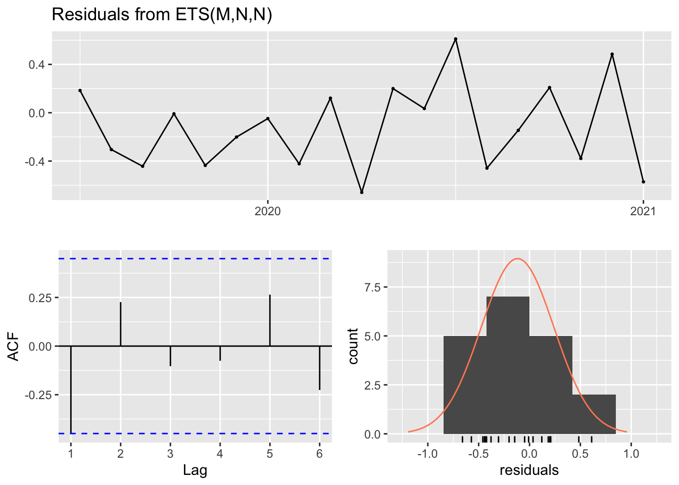

#> 
#>  Ljung-Box test
#> 
#> data:  Residuals from ETS(M,N,N)
#> Q* = 8.1278, df = 3, p-value = 0.04344
#> 
#> Model df: 2.   Total lags used: 5

And now we will plot the new predictions just like before.

users.ts.eol.predict = cbind(helix.users.eol,cadillac.users.eol)
dygraph(users.ts.eol.predict, main="Unique Users per Month (trained on EOL window)") %>% 
  dySeries("helix.users.eol", label="Helix") %>%
  dySeries("cadillac.users.eol", label="Cadillac") %>%
  dyAxis("y", label="Total jobs ended") %>%
  dyOptions(axisLineWidth = 1.5, fillGraph = TRUE) %>%
  dyShading(from="2021-02-02", to="2022-02-01", color = "#aad8e6") %>%
  dyRangeSelector()

This causes the prediction for Cadillac to tamper out, however our Helix prediction still has a non-stationary variance over time.

Predictive Analysis

Grouped Data Analysis

Monthly Datatables

Helix

Data Frame Summary

Cadillac

Data Frame Summary

Job Counts

Predictions using Error/Trend/Seasonality (ETS) Modeling

Job Count Predictions

ETS Models

Helix

Cadillac

Unique User Count Predictions

Users Model

Helix

Cadillac

Localized Models

Helix

Cadillac